The short answer
Keep the complete measured values and unit, declare every bin boundary and the rule for values on an edge, then compare plausible widths and starting offsets on the same data. A histogram groups observations; its tallest bar depends on that grouping. Preserve counts and outliers, and do not turn one attractive bin layout into a creator benchmark or content optimum.
What you’ll take away
- Bin width and starting offset are different choices.
- Every eligible value must enter exactly one bin.
- Show the original values and a sensitivity comparison beside the selected chart.
Ask a distribution question before selecting bins
After choosing a histogram to inspect a measured post-level distribution, specify the same response definition, observation age, period and selection across the data. A reaction count and a combined reactions-plus-comments count cannot silently share a column. Distinguish a distribution of posts from a distribution of creators; repeated posts can weight an author more heavily.
The earlier chart-selection guide chooses categories, time and genuine-whole relationships; the scale guide reviews numeric axes. This guide examines the separate grouping decision inside a histogram. NIST describes dividing a variable’s range into intervals and counting the observations in each. No grouping rule repairs a biased sample or unavailable measurements.
Write the edges and inclusion rule explicitly
Use a clear convention such as [left,right) for each bin, with the final right endpoint included. Under edges 0,10,20,30,40,50,60, a value of 20 belongs in [20,30), not the preceding bin; 60 belongs in the final [50,60]. The separate boundary probe includes 0,10,20,60 and confirms that none is dropped or counted twice.
Reject or explicitly handle values outside the declared range. An absent measurement is not zero, and an inconvenient high value is not an error merely because it stretches the picture. Record exclusions, units and the number of included values before counting. Keep full precision for assignment; round labels only after the bins are defined.
Reproduce three groupings of the same sixteen values
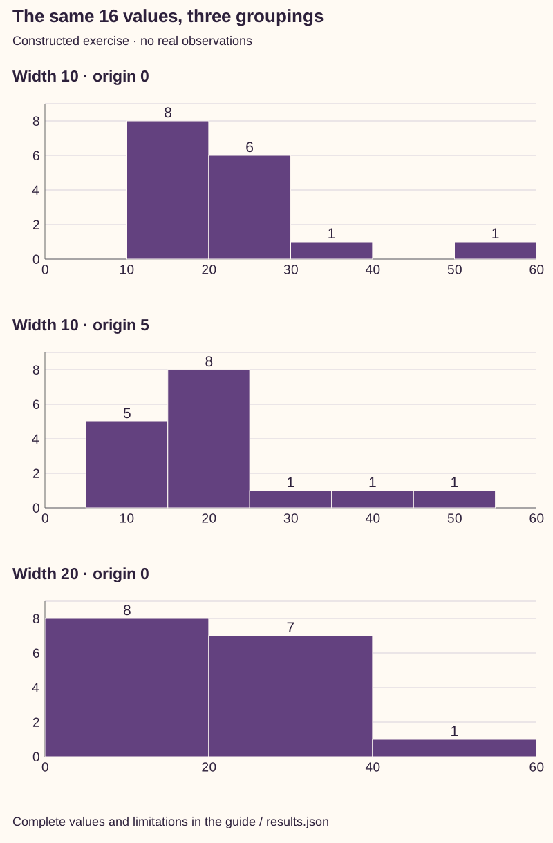
Our constructed responses are 10,11,12,13,14,16,18,19,20,21,22,23,24,25,38,52. Width 10 with origin 0 gives counts 0,8,6,1,0,1. Shifting the width-10 grid to origin 5 gives 5,8,1,1,1. Width 20 with origin 0 gives 8,7,1. Every layout retains all 16 values, including 38 and 52.
The largest bin is [10,20) in the first layout and [15,25) in the shifted one. Most values have not moved; the boundaries did. A claim that one narrow range is the creator’s uniquely typical performance would depend on the grouping. These fixtures are not real LinkedIn measurements or evidence of a population’s shape.
| Declared grid | Counts in increasing bin order | Included n |
|---|---|---|
| Width 10; edges 0 to 60 | 0 / 8 / 6 / 1 / 0 / 1 | 16 |
| Width 10; edges 5 to 55 | 5 / 8 / 1 / 1 / 1 | 16 |
| Width 20; edges 0 to 60 | 8 / 7 / 1 | 16 |
Keep bar height, relative count and density distinct
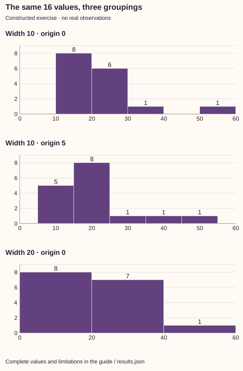
Our figures use equal-width bins within each panel and count on the vertical axis. A relative count divides a bin count by n. A density height instead divides by n times bin width, so area represents a fraction. NIST distinguishes those normalizations. If unequal widths are used, raw heights alone do not show equal fractions per unit width.
Label the scale and preserve bin widths when comparing graphics. A taller density bar after narrowing a bin is not automatically a larger group or greater total response. A histogram loses within-bin detail; use the full values, a dot display or a declared quantile when that detail is necessary. Do not infer an exact original observation from a bin midpoint.
Resolve three distribution readings
B1 — The tallest bar shifts after only the origin changes. Decision: retain both width-10 layouts and describe the concentration around the same underlying values. Result: a boundary-sensitive description, not changed creator performance.
B2 — A row equals 20 or the final edge 60. Decision: apply the declared half-open rule and final-edge exception, then check that total bin counts equal the included n. Result: exactly one assignment per supplied value, with no duplicated boundary response.
B3 — The high value 52 makes the tail look inconvenient. Decision: retain it unless a genuine source problem justifies a documented correction; inspect a different width without deleting it. Result: a reproducible sensitivity comparison, not a prettier chart obtained by removing an ordinary measured outcome.
Keep a grouping decision another person can reproduce
The worksheet keeps the reader question, source/unit/selection, full values, missingness, edges, inclusion rule, normalization, alternative layouts and chosen wording. The packet includes all values, three computed count vectors, both language figures and a standard-library checker with edge and out-of-range checks. No account connection or analytics upload is needed.
The relevant NIST histogram definitions and controls were read on 1 November 2026. All B-cases and values are constructed. Reproducing their counts establishes arithmetic only, not a universal bin rule, actual audience distribution, perception result or content effect.
Sources & product references
Product details reflect the publication date. External features and interfaces may change.